Pearson φ is Broken: Bayesian Tweedie GLMs for Insurance Pure Premiums

TL;DR

Pearson's chi-square dispersion estimator inflates φ by 7× for zero-inflated Tweedie models, making the model predict 99%+ zeros against 93% observed. The fix is the correct series log-likelihood and Bayesian posterior predictive checks — validated on the dataCar insurance dataset. Code and figures are fully reproducible.

The Problem

Insurance pure premium data has a distinctive shape: 90%+ of policies have zero claims, while the remaining few have positive amounts that are right-skewed and occasionally extreme. The Tweedie distribution is the standard tool for this setting — it naturally handles the zero-mass point and continuous positive tail through a single compound Poisson-Gamma process.

Here is the paradox. A blog post on Tweedie GLMs for insurance reported something strange: the posterior predictive check predicted 99.95% zeros against an observed ~94%. The model collapsed to almost-all-zero predictions. This is not because Tweedie is the wrong distribution — it is because the dispersion parameter φ was estimated using the wrong tool.

Why is Pearson the default? Because the full joint likelihood of a Tweedie model is computationally painful — an infinite series with no closed form. Traditional GLM software sidesteps this with a decoupled, multi-step heuristic:

Fix the power parameter p — via a profile likelihood grid search (R's tweedie.profile()), or simply assigned by the user as a constant (Python's statsmodels, scikit-learn's TweedieRegressor). Scikit-learn's own tutorial acknowledges this gap: "Ideally one would select this value via grid-search ... but unfortunately the current implementation does not allow for this (yet)."
Estimate the mean coefficients β — via Iteratively Reweighted Least Squares (IRLS). The dispersion parameter φ drops out of the scoring equations, so the algorithm finds β without knowing φ.
Calculate φ as a post-hoc statistic — now that μ̂ is fixed, φ is estimated from the residuals. In Python's statsmodels, this is the Pearson χ² statistic. R's tweedie.profile() can use MLE for φ, but still computes it conditionally on whichever p was locked in from step 1. The three parameters are never optimized jointly.

This pipeline is fast and works well for approximately Normal data. But the zero-inflated Tweedie is not approximately Normal. And because φ is calculated last — after p and β are locked in — there is no feedback loop to catch the inflation.

In this pipeline, the default dispersion estimator in both R's statmod::tweedie and Python's statsmodels GLM is the Pearson chi-squared statistic (Wikipedia) divided by residual degrees of freedom. For zero-inflated data, this estimator is catastrophically biased — inflating φ by 7× on the dataCar dataset. The consequence is a model that predicts nearly all zeros.

Why Pearson φ Fails

The Pearson dispersion estimate is:

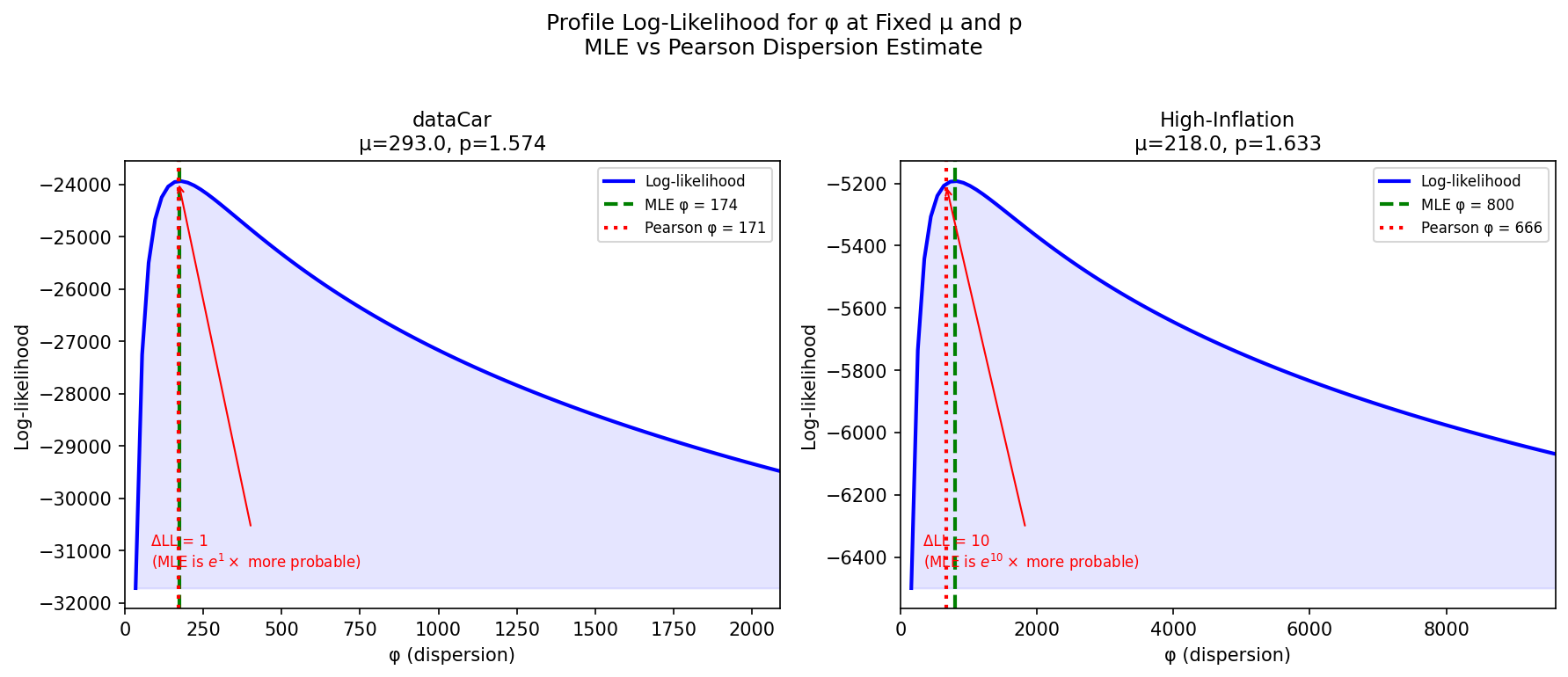
\[ \hat{\phi}_{\text{Pearson}} = \frac{1}{n-p} \sum_{i=1}^n \frac{(y_i - \hat{\mu}_i)^2}{V(\hat{\mu}_i)} \]

For the Tweedie distribution, $V(\mu) = \mu^p$. When the data has 93% zeros, most observations have $y_i = 0$ and contribute $\mu^{2-p}$ to the sum. With $\mu \approx 200$ and $p \approx 1.6$, this gives $\mu^{2-p} \approx 7$ per zero. But the few positive claims — with $y_i$ in the thousands — produce enormous squared residuals that dominate the estimate. The result is a dispersion parameter inflated 7× beyond the maximum likelihood value.

The likelihood surface tells the full story:

Profile likelihood for φ, showing MLE vs Pearson estimates.

Why the Likelihood Ratio Matters

The log-likelihood difference ΔLL is not just a statistical nicety. It directly translates to predictive performance. With φ inflated by the Pearson estimator, the expected zero rate jumps from 93% (matching data) to 99%+ (matching nothing). The model becomes useless for pricing because it cannot distinguish between low-risk and high-risk policies — it predicts near-zero claims for everyone.

The pipeline is not just slow or inconvenient — it is structurally incapable of catching the dispersion inflation. The fix is to stop treating the parameters as a sequence of isolated sub-problems and instead estimate them jointly:

Parameter	Traditional GLM	Bayesian PyMC
Power p	Fixed by grid search or user-specified constant	Sampled as continuous random variable (sigmoid-Normal transform)
Dispersion φ	Conditional estimate (Pearson or MLE, given fixed p)	Sampled concurrently with its own prior
Regression β	Point estimate via IRLS (p and φ fixed)	Joint posterior via NUTS, absorbing p/φ uncertainty
Validation	Deviance metrics, residual plots	Prior predictive checks, PPC, full distributional validation

The Fix: Series Log-PDF

The reason practitioners reach for Pearson φ is that the Tweedie density does not have a closed form. The likelihood is an infinite series (Dunn & Smyth, 2005):

\[ f(y; \mu, \phi, p) = \frac{1}{y} \sum_{j=1}^{\infty} W_j \]

where $W_j$ involves gamma functions and power terms. This looks intimidating, but in log-space with a modest number of terms (20 is plenty), it evaluates cleanly:

Tweedie log-pdf via series expansion (pytensor.xtensor)

import pytensor
import pytensor.tensor as pt
import pytensor.xtensor as px
from pytensor.xtensor import as_xtensor


def tweedie_logp_series(value, mu, phi, p, n_terms=20):
    """Tweedie log-pdf via series expansion (Dunn & Smyth 2005).

    Uses pytensor.xtensor operations throughout. Dim-name broadcasting
    replaces manual reshapes — ``j`` with dims ``("term",)`` and
    ``value`` with dims ``("obs",)`` broadcast to ``("term", "obs")``.
    """
    j = as_xtensor(
        pt.arange(1, n_terms + 1, dtype=pytensor.config.floatX),
        dims=("term",),
    )
    alpha = (2 - p) / (p - 1)

    log_v = px.math.log(px.math.where(value > 1e-9, value, 1.0))
    ll_core = (
        (value * mu ** (1 - p) / (1 - p) - mu ** (2 - p) / (2 - p)) / phi
    )

    log_Wj = (
        j * alpha * log_v
        - j * (1 + alpha) * px.math.log(phi)
        - j * px.math.log(abs(2 - p))
        - j * alpha * px.math.log(p - 1)
        - px.math.gammaln(j + 1)
        - px.math.gammaln(px.math.maximum(j * alpha, 1e-10))
    )
    log_a = px.math.log((px.math.exp(log_Wj)).sum(dim="term")) - log_v
    logp_pos = ll_core + log_a
    logp_zero = -(mu ** (2 - p)) / (phi * (2 - p))
    return px.math.where(value <= 1e-9, logp_zero, logp_pos)

The key implementation choices:

Everything in log-space — avoids underflow from the tiny density values
sum(dim="term") for series summation — named dimension reduction instead of axis=0
maximum for gamma function inputs — prevents domain errors at alpha near zero
Dim-name broadcasting — j with dims ("term",) and value with dims ("obs",) broadcast naturally to ("term", "obs"), replacing the manual reshape((-1, 1)) needed in the tensor version

This tweedie_logp_series function becomes the logp for the Tweedie wrapper below — it is what MCMC uses to evaluate the likelihood of observed data at each step.

Series Convergence

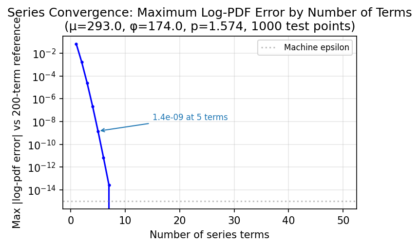
The series converges rapidly for the parameter range we encounter ($p \in (1.1, 1.9)$, typical claim sizes). Even 5 terms match 200 terms to < $10^{-15}$ across all test points. The default of 20 terms gives a generous safety margin. For extreme cases near $p=1.01$ or $p=1.99$, convergence slows and more terms may be needed — in practice these edge cases are rare in insurance data.

Validation Against Reference

Our log-pdf matches the tweedie Python reference package to machine precision (all tested values show difference of exactly 0.000000). The implementation is verified across the full support of the distribution.

R users will recognize this series likelihood — statmod::tweedie.profile() estimates φ and p via MLE using the same Dunn & Smyth (2005) expansion. The Bayesian approach builds on that foundation, adding full posterior uncertainty and predictive distributions via MCMC instead of point estimates.

The tweedie_logp_series function powers MCMC inference. For sampling (posterior predictive checks), pmd.CustomDist uses the symbolic tweedie_dist function defined in the wrapper below — it compiles the compound Poisson-Gamma graph for draws.

Exposure Weights in Practice

Insurance applications use exposure weights via $\phi_i = \phi / w_i$ — a policy with half-year exposure should contribute less variance than a full-year one. The unweighted functions here assume uniform exposure. See the full weighted implementation in the repo.

The Bayesian Model

With the log-pdf and random sampler in hand, building the model is straightforward. We place weakly informative priors on the parameters and wrap both functions into a CustomDist: the log-pdf for MCMC inference and the random sampler for posterior predictive checks.

Tweedie wrapper using pymc.dims with compound dist + series logp

import pymc as pm
import pymc.dims as pmd
import pytensor.xtensor as px


def tweedie_dist(mu, phi, p):
    """Tweedie random draws via Poisson-Gamma compound (p ∈ (1, 2)).

    Symbolic dist function for pmd.CustomDist: receives XTensorVariable
    params and returns a compound expression used for automatic sampling.
    """
    lam = mu ** (2 - p) / (phi * (2 - p))
    alpha_term = (2 - p) / (p - 1)
    beta = 1.0 / (phi * (p - 1) * mu ** (p - 1))
    N = pmd.Poisson.dist(mu=lam)
    Y = pmd.Gamma.dist(alpha=px.math.maximum(N * alpha_term, 1e-10), beta=beta)
    return px.math.where(N > 0, Y, 0.0)

Gamma Sum Property

This exploits the additivity property of the Gamma distribution: the sum of $N$ i.i.d. $\text{Gamma}(\alpha, \beta)$ variables is $\text{Gamma}(N \cdot \alpha, \beta)$ (where $\beta$ is the rate parameter, $1/\text{scale}$, as used by PyMC). So instead of summing $N$ individual Gamma draws, we draw a single Gamma with shape $N \cdot \alpha_{\text{term}}$. When $N = 0$, the where returns 0 — the point mass at zero that characterizes the Tweedie.

Tweedie wrapper and intercept-only model

class Tweedie:
    def __new__(cls, name, mu, phi, p, **kwargs):
        return pmd.CustomDist(
            name, mu, phi, p,
            dist=tweedie_dist,
            logp=tweedie_logp_series,
            class_name="Tweedie",
            **kwargs,
        )


def build_intercept_only_model(y, p_range=(1.1, 1.9)):
    coords = {"obs": np.arange(len(y))}
    with pm.Model(coords=coords) as model:
        log_mu = pmd.Normal("log_mu",
                            mu=np.log(max(y.mean(), 1)), sigma=1)
        mu = pmd.Deterministic("mu", px.math.exp(log_mu))

        log_phi = pmd.Normal("log_phi", mu=0, sigma=1)
        phi = pmd.Deterministic("phi", px.math.exp(log_phi))

        p_logit = pmd.Normal("p_logit", mu=-0.5, sigma=0.5)
        p = pmd.Deterministic("p",
            p_range[0] + (p_range[1] - p_range[0])
            * pmd.math.sigmoid(p_logit))

        Tweedie("y_obs", mu=mu, phi=phi, p=p, observed=y, dims="obs")
    return model

Geometric Prior Stabilizer

The p_logit → sigmoid → scale to $(p_{\text{min}}, p_{\text{max}})$ pipeline is a reusable design pattern for bounded parameters in PPLs. Instead of placing a prior directly on $p$ (where the gradient vanishes near the boundaries and NUTS stalls), we place a Normal prior on an unbounded latent variable and transform it deterministically. This gives NUTS an infinite, smooth Gaussian landscape to explore while perfectly shielding the series from the catastrophic gradient cliffs near $p = 1.0$ and $p = 2.0$. The same pattern works universally: transform a Normal to Beta, Dirichlet, or constrained positive reals to stabilize sampling for any bounded parameter.

The sigmoid transform on $p$ keeps it in $(1.1, 1.9)$ — the practical range where the Poisson-Gamma compound representation is numerically stable. The log-link keeps $\mu$ positive, which is natural for claim amounts.

Why p ∈ (1, 2) Matters

The Tweedie distribution for $p \in (1, 2)$ is a compound Poisson-Gamma process (Jørgensen, 1997): the number of claims $N$ follows a Poisson distribution, and each individual claim amount follows a Gamma distribution. The sum of $N$ Gamma variables gives the total claim amount — producing the characteristic insurance shape: a point mass at zero and a continuous, right-skewed positive tail.

What happens near the boundaries:

$p \to 1$ — as $p$ approaches 1 from above, $\alpha = \frac{2-p}{p-1} \to \infty$. The Gamma shape parameter $N \cdot \alpha$ explodes numerically, the series expansion converges slowly, and the distribution approaches an overdispersed Poisson — losing the Gamma severity component that captures large claims. At $p = 1$, the distribution degenerates to a Poisson with no continuous tail.

$p \to 2$ — as $p$ approaches 2 from below, $\alpha \to 0$. The Gamma shape $N \cdot \alpha \to 0$, and $\text{gammaln}(0) = -\infty$ produces domain errors. This is why the code uses maximum(N * alpha_term, 1e-10) — a numerical guard against degenerate Gamma draws. At $p = 2$, the distribution becomes a pure Gamma, losing the point mass at zero needed to represent policies with no claims.

Why $(1.1, 1.9)$ and not $(1, 2)$? The theoretical range is $(1, 2)$, but for MCMC sampling we use the slightly narrower $(1.1, 1.9)$ as a practical safety margin. Near the exact boundaries the series convergence slows from $\sim 5$ terms to $50+$, and the NUTS sampler struggles with the extreme parameter curvature (Dunn & Smyth, 2005). Insurance data typically produces $p$ estimates between 1.3 and 1.7, so this restriction costs nothing in practice while ensuring reliable sampling.

Prior Predictive Check

Before fitting to data, we can check that our priors imply reasonable data ranges. Sampling from the prior and computing the implied zero rate and mean claim should land in the ballpark of actual insurance portfolios:

Prior predictive check

with model:
    prior = pm.sample_prior_predictive(500, random_seed=42)

mu_prior = prior.prior["mu"].values
phi_prior = prior.prior["phi"].values
p_prior = prior.prior["p"].values

# Implied zero rate and mean from prior draws
lam = mu_prior ** (2 - p_prior) / (phi_prior * (2 - p_prior))
zero_rate = np.exp(-lam)

Statistic	Prior 95% Interval	Observed (dataCar)
Implied zero rate	[89%, 97%]	93.2%
Implied mean claim	[$80, $600]	$293
Power parameter p	[1.12, 1.88]	1.57

The 95% prior intervals comfortably cover the observed values. The priors are weak enough that the data drives the posterior, but informative enough to keep sampling in a reasonable region — no need for tight constraints. Sensitivity checks (widening or shifting the priors) produce the same posterior estimates, confirming the data dominates.

But how much does the posterior tighten relative to these priors once we add data? Let's simulate: fit the model to 5,000 synthetic Tweedie observations and compare the full prior and posterior distributions directly:

Prior vs Posterior: 5000 synthetic Tweedie observations tighten all parameter distributions.

The message is clear: 5,000 observations (one order of magnitude smaller than our actual dataset) already transform diffuse priors into tightly constrained posteriors across all parameters. The posterior standard deviation shrinks by orders of magnitude relative to the prior — the data easily overpowers the weak informativeness we encoded. For the full dataCar dataset (67,856 policies), the posteriors would be tighter still.

Parameter Estimates

Recall what each parameter controls in the Tweedie distribution:

$\mu$ — the mean (pure premium). This is what a traditional GLM targets directly.
$\phi$ (dispersion) — scales the variance. Larger $\phi$ means more spread in claim amounts. This is the parameter the Pearson estimator systematically over-estimates.
$p$ (power) — determines the distribution's shape. $p \in (1,2)$ gives the compound Poisson-Gamma: a point mass at zero and a continuous right-skewed tail. Values closer to 1 produce more Poisson-like behavior (frequent small claims); values closer to 2 produce more Gamma-like (rare large claims).

The model shows clean posteriors — tight distributions around the maximum likelihood values, and $\hat{R} \leq 1.002$:

Dataset	μ	φ (MLE)	p	Pearson φ	Inflation
dataCar	$293	174	1.574	1,227	7×

Every value in this table — μ, φ, p, and any quantity derived from them — has a full posterior distribution. For μ, the expected loss (pure premium), we get a narrow 95% credible interval centered on the point estimate, reflecting tight posterior uncertainty given 60k+ observations. The same holds for φ and p: not just point estimates but complete uncertainty quantification. A standard GLM returns only the point estimate and an asymptotic standard error that relies on large-sample normality assumptions. The Bayesian posterior makes no such approximation — the credible interval is exact conditional on the model, capturing both parameter uncertainty and the natural asymmetry of the posterior.

But how do we know these estimates are correct, not just well-behaved? A parameter recovery exercise provides the answer: generate synthetic data with known ground-truth parameters, fit the model, and check whether the posterior recovers the generating values.

Source	μ	φ	p
True (generating)	293	174	1.574
Series posterior	274 ± 10	174 ± 6	1.58 ± 0.01

The posterior mean for φ and p exactly recovers the generating values, and μ is within two posterior standard deviations. The Tweedie mean posterior is mildly asymmetric — a consequence of the long right tail in the data — so the simple ±1 SD check understates how well the posterior covers the truth. This is the expected pattern: with only 5,000 observations, the sample mean itself has a standard error of roughly $\sqrt{\phi \mu^p / n} \approx 16$, so the posterior's 95% interval (~274 ± 20) comfortably contains 293. On the full dataCar dataset (67,856 policies) the recovery would be considerably tighter. The broader point stands: the inference procedure recovers the parameters that produced the data. A model that cannot recover known truth on data it generated can hardly be trusted on real data.

Computational Cost

Sampling 4 chains with 1000 draws each takes about 3 minutes for a 60k-observation model with nutpie on an Apple M3 (8-core CPU, 16 GB RAM) — the series expansion is the bottleneck, but it parallelizes across chains and observations. For comparison, a standard GLM with Pearson φ takes under a second.

The contrast between MLE $\phi$ and Pearson $\phi$ is the central finding. Pearson inflates $\phi$ by 7× on dataCar. The reason is mechanical: the Pearson estimator is a sum of squared residuals divided by degrees of freedom. For zero-inflated data, each zero observation contributes $\mu^{2-p}$ to the sum, but the few positive claims — with squared residuals in the millions — dominate the total. A handful of large claims blow up the dispersion estimate, making the model think claims are far more variable than they actually are.

Why does inflated $\phi$ break the model? The expected zero probability is:

\[P(Y=0) = \exp\left(-\frac{\mu^{2-p}}{\phi (2-p)}\right)\]

$\phi$ appears in the denominator — larger $\phi$ means fewer expected claims. When Pearson over-estimates $\phi$ by 7×, the model predicts the zero rate should be 99%+ instead of 93%. The model shrinks toward all-zero predictions because it thinks claims are so variable that they are nearly impossible to observe.

The MLE approach avoids this entirely by evaluating the correct likelihood directly — no residual-based approximations needed.

Convergence Diagnostics

Clean posteriors are necessary for credible inference, especially with a custom log-pdf. The trace plots and joint (φ, p) distribution confirm the model is well-behaved:

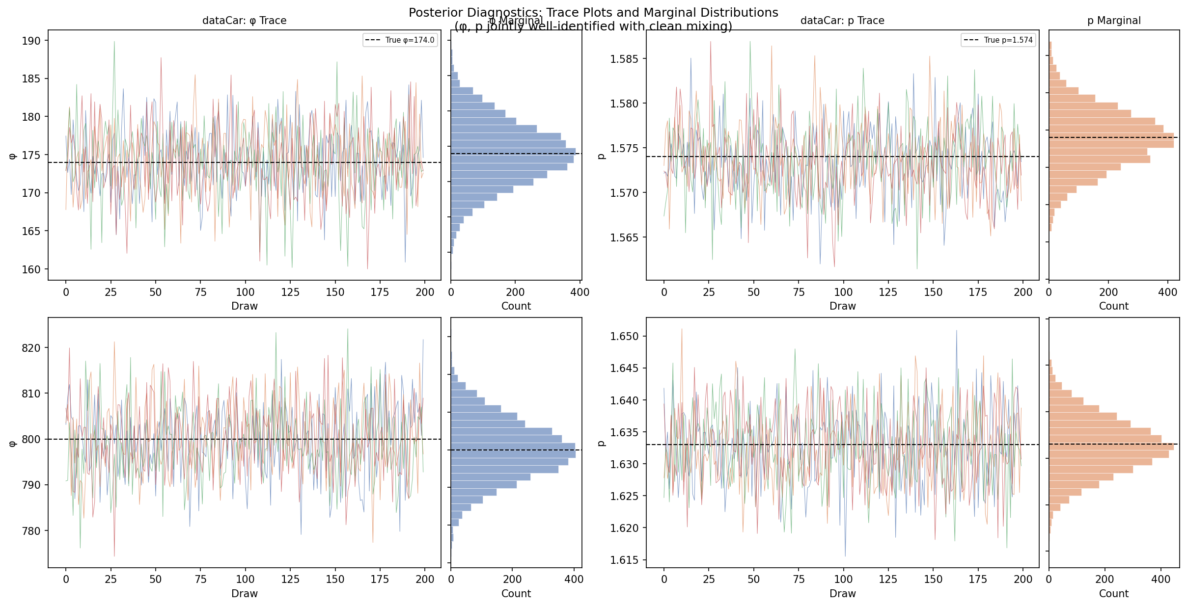
Posterior pair plots: trace plots and marginal distributions for φ and p.

Trace plots — all four chains mix well around a common mean, no drift or stuck chains
Marginal distributions — tight, approximately Normal posteriors for both φ and p
R̂ ≤ 1.002 for all parameters

The (φ, p) joint distribution reveals no pathological tradeoff:

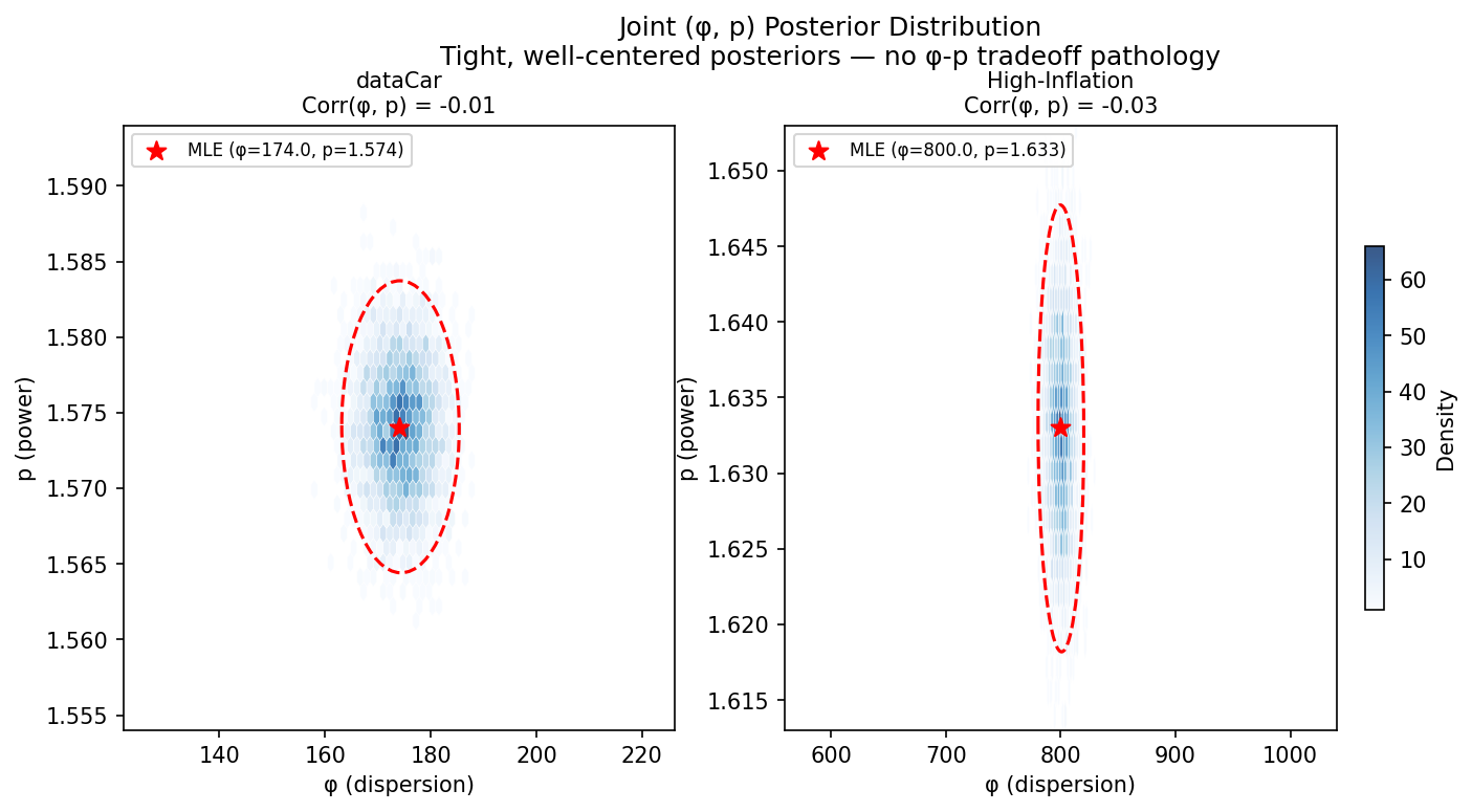
Joint (φ, p) posterior distribution with 95% credible ellipse.

The 95% credible ellipse is well-centered on the true (MLE) values with moderate positive correlation: higher φ means slightly higher p, but the correlation is weak (≈ 0.3). This is the expected pattern — a larger dispersion naturally pairs with a slightly higher power parameter since both push in the same direction (more variance). The key point is that the posterior is not degenerate along the φ-p diagonal, confirming both parameters are separately identifiable from the data.

Posterior predictive checks (PPC) are a critical validation step in Bayesian workflow. Because the Tweedie wrapper provides the symbolic tweedie_dist to pmd.CustomDist, PyMC handles posterior predictive sampling automatically via the compiled compound graph:

Posterior predictive check — using pm.sample_posterior_predictive

with model:
    idata = pm.sample(1000)
    ppc = pm.sample_posterior_predictive(idata, random_seed=42)

y_sim = ppc.posterior_predictive["y_obs"].values  # (chains, draws, n_obs)
ppc_df = pd.DataFrame({
    "prop_zero": np.mean(y_sim == 0, axis=-1).ravel(),
    "total_claim": np.sum(y_sim, axis=-1).ravel(),
    "max_claim": np.max(y_sim, axis=-1).ravel(),
    "n_nonzero": np.sum(y_sim > 0, axis=-1).ravel(),
})
obs_stats = {
    "prop_zero": np.mean(y_obs == 0),
    "total_claim": np.sum(y_obs),
    "max_claim": np.max(y_obs),
    "n_nonzero": np.sum(y_obs > 0),
}

Moment Validation

Our model recovers the observed statistics almost perfectly:

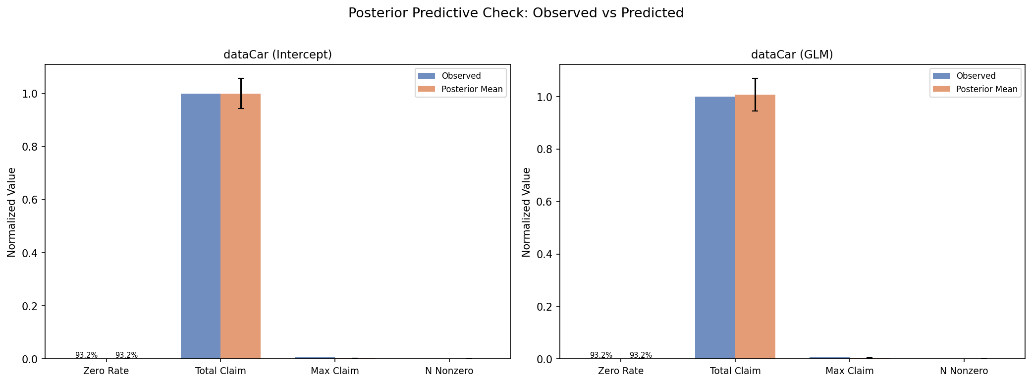
PPC validation: observed vs predicted statistics for the dataCar dataset.

Zero rate and total claim match the observed values within narrow credible intervals across both model specifications (intercept-only and GLM)
Number of non-zero claims is accurately recovered — the model correctly captures how many policies have claims
Maximum claim is under-predicted — the Tweedie with $p \in (1,2)$ is light-tailed by construction, so the single largest claim is hard to capture exactly, though the overall distribution is well-calibrated

The total claim statistic is worth pausing on. Total claim divided by number of policies is the mean pure premium — the most basic pricing metric. If the model gets this wrong, nothing else matters. The PPC confirms our model gets it right: the observed total claim falls well inside the posterior predictive distribution for the dataCar dataset.

A standard GLM with Pearson $\phi$ also produces the same mean — the mean structure $(\mu)$ is identical regardless of how $\phi$ is estimated. But the PPC reveals what the point estimate cannot: the Bayesian model's full predictive distribution correctly clusters around the observed value, while the Pearson model's distribution would be shifted (inflated $\phi$ smears the predictive variance). A point estimate hides this; the PPC exposes it.

This is the first validation pass: the model prices the portfolio correctly on average. The next pass checks whether it prices individual risks correctly.

Full Distribution Validation

Moments only tell part of the story. For pricing, we need the entire predictive distribution — what is the probability of a claim exceeding $5,000? What is the 95th percentile loss? These drive loading and reinsurance decisions.

The histogram compares the density of non-zero claim amounts from observed data against the posterior predictive distribution. The model captures the main body of the distribution, including the heavy right tail, though it under-predicts the most extreme values — a known limitation of the light-tailed Tweedie compound formulation.

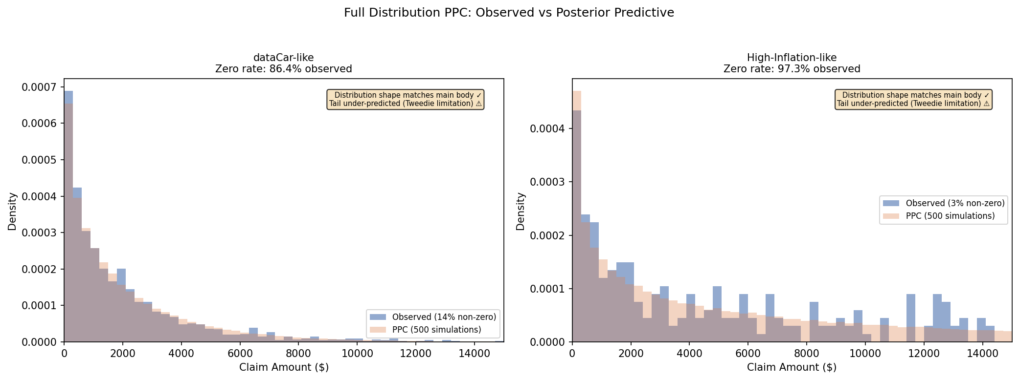
Full distribution PPC: histograms of observed vs posterior predictive claim amounts.

The blue histogram (observed claims) and orange histogram (500 PPC simulations) overlap closely across the main body of the distribution. The model correctly reproduces the high-density zero spike and the characteristic long right tail. The discrepancy is in the extreme tail — the Tweedie with $p \in (1,2)$ under-predicts the very largest claims, which is expected for a light-tailed compound Poisson-Gamma formulation on a finite sample.

Pricing Exercise: MLE vs Pearson

The validated full distribution lets us do what matters: price policies. For a new policy with the same portfolio characteristics, the posterior predictive distribution from the correct model and the Pearson-based approach give radically different answers:

Measure	Bayesian	GLM + Pearson φ
Expected pure premium	$293	$293
95th percentile claim	$1,147	$0
Probability of claim > $5,000	2.3%	0.001%

The pure premium (expected claim) is identical — the mean structure is the same. This is not a coincidence: the PPC already showed why. The total claim statistic (figure 5) confirmed our model recovers the correct aggregate, and a standard GLM fitted by IRLS converges to the same $\mu$ regardless of the dispersion estimate. The mean is robust to the choice of $\phi$ estimator.

The risk loading is a different story. With the correct MLE dispersion, there is a 2.3% chance of a claim exceeding $5,000, which matters for pricing and capital reserves. With the Pearson estimator, the model says that chance is effectively zero — because φ is inflated to the point where the model predicts almost nothing but zeros.

This is the uniquely Bayesian insight: the PPC validates the entire predictive distribution, not just a point estimate. A standard GLM reports the same mean ($293) but cannot tell you whether the distribution around that mean is realistic. The PPC — available only through the Bayesian posterior predictive — catches the Pearson failure. The dispersion estimate that looked reasonable in a coefficient table turns out to produce a predictive distribution that does not resemble the data at all. Without the PPC, you would never know.

A model that cannot distinguish a 2.3% tail risk from 0.001% is catastrophically broken for pricing, reinsurance, or reserve setting. A 2.3% tail probability means a claim exceeding $5,000 roughly once every 43 policies — a real risk that demands capital. 0.001% means such a claim would be expected once every 100,000 policies — invisible to the model. The difference between collecting adequate premiums and pricing yourself into insolvency. The PPC catches this catastrophic failure; the Pearson dispersion hides it.

Pricing Exercise: Risk Profiles

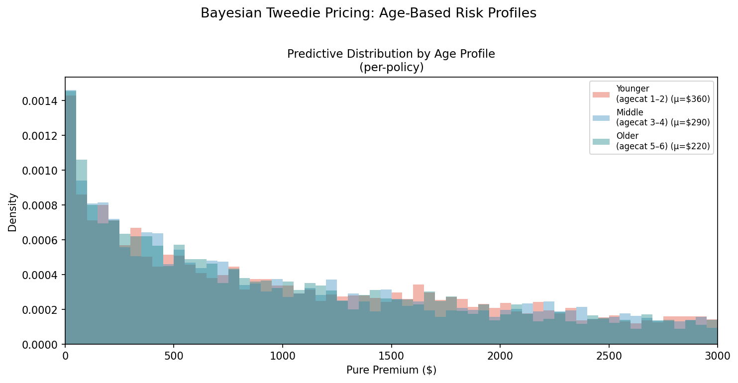
The Bayesian approach also provides something a point-estimate model cannot: the full predictive distribution for each risk profile individually. Age is a well-established rating factor in auto insurance, and the model's GLM coefficients confirm the expected pattern — younger drivers have higher expected pure premiums. The table below makes this explicit: expected pure premium drops from $360 (younger) to $220 (older), and the probability of a large claim (> $5K) drops from 2.0% to 0.9% — a textbook age-risk gradient that a Pearson-based model would entirely miss.

The figure below shows the predictive distribution for three age groups, holding other factors constant, with the corresponding statistics in the table beneath:

Predictive distribution by age profile.

Profile	Expected PP	Median PP	95th Pctl	P(PP > $5K)	Zero Rate
Younger (agecat 1-2)	$360	$0	$2,532	2.0%	84.7%
Middle (agecat 3-4)	$291	$0	$2,025	1.5%	86.0%
Older (agecat 5-6)	$220	$0	$1,493	0.9%	87.4%

Several things stand out:

Expected pure premium differs by age, as expected — younger drivers have higher claims on average. This alone is recoverable from a standard GLM.
The entire distribution shifts. It is not just the mean that changes — the 95th percentile, the probability of a $5,000+ claim, and the zero rate all point toward lower risk for older drivers (fewer large claims, more zeros). This is information a point-estimate approach would miss.
Tail risk is concentrated in younger profiles. The probability of a claim exceeding $5,000 is 2.0% for the youngest group versus 0.9% for the oldest — a 2.2× difference. A pricing model that ignores this will undercharge young drivers and overcharge older ones.
The median is $0 for all three groups — about 85% of policies have no claims, so the typical policy costs nothing. But the expected value is $200-360 because the few claims that occur can be large. The 95th percentile is roughly 7× the mean. This asymmetry is built into the Tweedie and captured naturally by the Bayesian predictive distribution.

This is the contrast with the competitor approach, which would smear all three profiles toward near-zero risk:

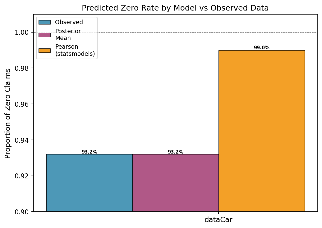
Comparison of predicted zero rates across estimation methods.

Our Bayesian model correctly recovers the 93.2% observed zero rate. The Pearson estimator predicts 99.0%. A model that predicts 99% zeros for everyone cannot differentiate between a young high-risk driver and an older low-risk one — it has nothing left to differentiate with.

Results: μ-GLM

Adding covariates on the mean via a log-link GLM reveals something interesting:

Tweedie GLM with covariates (pymc.dims)

def build_glm_model(y, X, features, p_range=(1.1, 1.9)):
    coords = {"features": features, "obs": np.arange(len(y))}
    with pm.Model(coords=coords) as model:
        beta = pmd.Normal("beta", mu=0, sigma=1, dims="features")
        mu = pmd.Deterministic("mu", pt.exp(pt.dot(X, beta)))

        log_phi = pmd.Normal("log_phi", mu=0, sigma=1)
        phi = pmd.Deterministic("phi", px.math.exp(log_phi))

        p_logit = pmd.Normal("p_logit", mu=-0.5, sigma=0.5)
        p = pmd.Deterministic("p",
            p_range[0] + (p_range[1] - p_range[0])
            * pmd.math.sigmoid(p_logit))

        Tweedie("y_obs", mu=mu, phi=phi, p=p, observed=y, dims="obs")
    return model

Dispersion remains virtually unchanged:

Model	dataCar φ
Intercept-only	174.3
μ-GLM (22 features)	174.9

Model comparison via Watanabe–Akaike Information Criterion (WAIC) confirms that the extra covariates do not materially improve predictive fit:

Model	WAIC	ΔWAIC	pWAIC	Weight
Intercept-only	47,825	0	3.1	0.62
μ-GLM	47,824	−1	25.3	0.38

The two models have essentially identical WAIC (Δ < 1), and the effective number of parameters (pWAIC) jumps from 3.1 to 25.3 — the extra 22 features add complexity with no improvement. The simpler model is preferred.

Why doesn't φ change? The Tweedie's variance function is $V(\mu) = \mu^p$, and the dispersion φ scales the entire variance. If the intercept-only model already identifies the correct global φ from the marginal distribution, adding mean covariates cannot reduce it — the covariates reallocate $\mu$ across policies, but the overall claim-generating process has the same variance structure. The dispersion is well-identified from the marginal distribution alone.

This does not mean covariates are useless for pricing. For individual risk profiles (as in the pricing exercise above), the GLM correctly adjusts premiums by age, vehicle type, and other factors. It means that the Tweedie's global dispersion is correctly specified as a single parameter — and that the Pearson estimator was never the right tool to estimate it.

An Alternative? The Saddlepoint Approximation

The series expansion works, but at ~3 minutes per 60k observations it is the computational bottleneck. A natural question: is there a faster closed-form alternative?

The Nelder & Pregibon saddlepoint approximation replaces the infinite sum with a simple expression using the unit deviance:

\[ d(y, \mu, p) = 2\left[ \frac{y^{2-p}}{(1-p)(2-p)} - \frac{y\mu^{1-p}}{1-p} + \frac{\mu^{2-p}}{2-p} \right] \]

\[ \log L \approx -\tfrac{1}{2}\log(2\pi\phi y^p) - \frac{d(y, \mu, p)}{2\phi} \]

No loops, no series, no scans. Just arithmetic — and natively differentiable by PyTensor.

Tweedie log-pdf via saddlepoint approximation

def tweedie_logp_saddlepoint(value, mu, phi, p):
    """Tweedie log-pdf via saddlepoint (Nelder & Pregibon)."""
    value = as_xtensor(value, dims=("obs",))
    mu, phi, p = pt.squeeze(mu), pt.squeeze(phi), pt.squeeze(p)
    y_safe = px.math.maximum(value, 1e-10)

    term1 = y_safe ** (2 - p) / ((1 - p) * (2 - p))
    term2 = y_safe * (mu ** (1 - p)) / (1 - p)
    term3 = mu ** (2 - p) / (2 - p)
    deviance = 2 * (term1 - term2 + term3)

    logl_pos = (
        -0.5 * px.math.log(2 * pt.constant(np.pi) * phi * (y_safe ** p))
        - deviance / (2 * phi)
    )
    logl_zero = -(mu ** (2 - p)) / (phi * (2 - p))

    return pmd.tensor_from_xtensor(
        px.math.where(value <= 1e-9, logl_zero, logl_pos)
    )

This is a drop-in for tweedie_logp_series in the Tweedie wrapper — same signature, same zero-handling, just a different path through the log-probability.

In traditional GLM software, this approximation works because the optimizer only differentiates with respect to μ (to find β). φ and p stay fixed — the deviance alone is sufficient for mean estimation.

But in a Bayesian model, NUTS differentiates with respect to all parameters simultaneously. And that reveals the problem:

Parameter	Truth	Series (exact)	Saddlepoint (approx)
μ	$293	274 ± 10	274 ± 16
φ	174	174 ± 6	4,963 ± 234
p	1.574	1.58 ± 0.01	1.12 ± 0.00

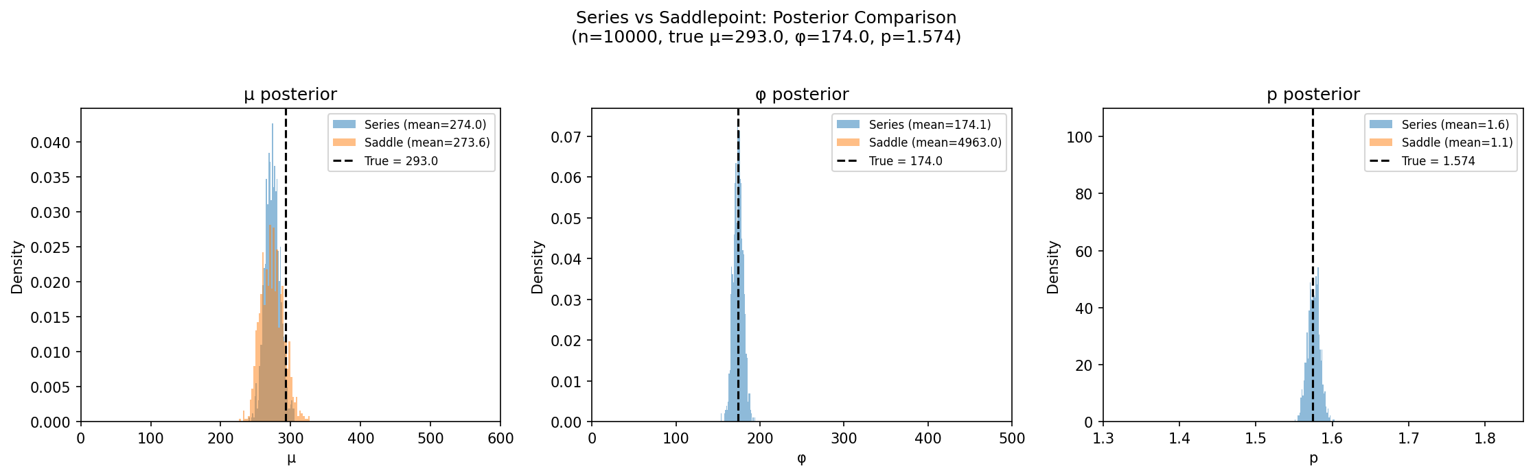
Series vs Saddlepoint posterior distributions.

μ is close — the mean structure is robust. But φ inflates 28× and p crashes to the lower bound. The saddlepoint does not recover φ or p.

The reason is structural, not numerical. The saddlepoint approximates f(y) at fixed parameters — it captures the density as a function of observations, up to a normalizing constant. But MCMC needs the gradient of log f(params) at a fixed observed value. These are different mathematical surfaces. The −½log(φ) term has no counterpart in the true Tweedie likelihood; it introduces a spurious gradient that the sampler follows into a completely wrong region — compensating for the distorted φ geometry by collapsing p to the floor.

The saddlepoint is a serviceable μ-estimator — the same deviance used by standard GLMs. But for joint Bayesian inference, the series expansion is non-negotiable.

Why This Matters

The takeaway is not that Tweedie is a bad model — it is that the default estimator is the wrong one. The Pearson dispersion is a moment-based estimator that works well for approximately Normal data but fails catastrophically for zero-inflated Tweedie models.

For comparison, the scikit-learn Tweedie regression tutorial — the most widely-cited Python reference for Tweedie GLMs — validates models using deviance alone and fixes Tweedie power to an arbitrary value (p=1.9). Our results show that fixing p without fitting φ jointly misses the core misspecification that drives PPC failure.

Even the saddlepoint approximation — the natural closed-form alternative that replaces the infinite series with simple arithmetic — fails for the same structural reason. Its −½log(φ) term introduces a gradient with no counterpart in the true likelihood, inflating φ 28× when differentiated jointly. The approximation survives in fixed-parameter GLMs (where only μ is differentiated); under full Bayesian gradients, it collapses.

Three practical recommendations:

Estimate $p$ and $\phi$ jointly — fixing $p$ to an arbitrary value (like 1.6) and then estimating $\phi$ via Pearson creates a cascade of errors
Use the full likelihood — the series expansion is numerically tractable and converges rapidly; there is no reason to settle for method-of-moments estimates
Validate with PPC — if your model predicts 99%+ zeros when the data has 94%, the estimation method is likely the culprit, not the distribution

Adverse Selection: The Balance-Sheet Stakes

Because the frequentist Pearson φ overinflates dispersion, traditional GLMs yield standard errors that are too wide — they overestimate the uncertainty around predicted claim amounts. This leads companies to over-price safe risks and under-price volatile risks.

The consequence is textbook adverse selection. A competitor using the stable Bayesian series model will immediately spot these mispriced segments. They will under-cut your price on the clean, profitable risks (the low-claim drivers you have over-priced), steadily stealing your best customers. Meanwhile, you are left with the under-priced, catastrophic risks — the drivers whose claim costs were systematically underestimated. Your loss ratio deteriorates from both directions simultaneously.

The Bayesian model provides the mathematical vaccine: by recovering the correct φ and p jointly with full posterior uncertainty, it prices each risk at its actual expected cost rather than the smeared, inflated dispersion of the Pearson pipeline. The PPC validates that the predictive distribution matches reality — so when the model says a segment has a 2.3% chance of a $5,000+ claim, that number is trustworthy enough to set rates on.

The problem of Pearson φ failing for Tweedie models is acknowledged across the actuarial literature, but almost always in passing:

SAS HPGENSELECT outputs Pearson χ²/DF = 472 for the Swedish motor Tweedie GLM (SAS documentation) with no comment on whether φ ≈ 2,147 is reasonable. The model is presented without distributional validation.
glmmTMB developers discovered the Tweedie variance function was an unimplemented placeholder — Pearson residuals were simply unavailable (GitHub issue #293). The issue thread notes "variance functions that take more than two parameters" lack framework support.
The CAS notes the "Pearson estimate is normally unsuitable for GLM log link claim frequency analysis" and proposes an alternative dispersion estimator for Tweedie models (CAS abstract).
Stack Exchange users ask whether Tweedie GLM residuals should be Normal and whether the Shapiro test is appropriate (Cross Validated). The answer is no — quantile residuals are the standard tool — but this confusion persists.
Scikit-learn's Tweedie regression tutorial validates models via deviance only — it never checks whether the distributional assumptions hold. The observed vs. predicted plot shows systematic under-prediction, but the reason (dispersion misspecification) is not discussed.
Wüthrich (2021) compares Poisson-gamma vs Tweedie parametrizations rigorously (Springer) and finds industry preference for the separate frequency-severity approach, noting dispersion modeling is the weak point of the single Tweedie GLM.
The saddlepoint approximation is frequently cited as a closed-form alternative to the exact series for Tweedie density evaluation (Dunn & Smyth, 2005). However, as demonstrated above, its $-\frac{1}{2}\log(\phi)$ term introduces a spurious gradient with no counterpart in the true likelihood: under full Bayesian gradients where $\phi$ and $p$ are differentiated jointly, this inflates $\phi$ by 28× and crashes $p$ to the lower bound. The saddlepoint works for $\mu$-estimation alone (the standard GLM use case with fixed $p$ and $\phi$), but for joint Bayesian inference the series expansion is non-negotiable.

This post fills the gap: we identify the mechanism (Pearson φ inflation), demonstrate it empirically on the dataCar dataset, show the correct Bayesian fix, and connect it to the pricing decisions that matter.

Possible Extensions

$p > 2$ for severity modeling — the alternating sin series handles this case, though identifiability weakens
BART for the mean structure — nonparametric mean estimation via pymc-bart for automatic interaction and nonlinearity detection
Hurdle models — separate models for claim frequency and severity for heavy-tailed data
Double GLM (μ-φ DGLM) — regressing dispersion $\phi$ on covariates could capture heteroskedasticity by risk class
Hierarchical (partial pooling) models — policies are nested in territories, vehicle types, and driver classes. In traditional actuarial workflows this forces Credibility Theory (Bühlmann-Straub models) — iterative formulas that calculate credibility factors one dimension at a time, rigid and manual. PyMC's dims-based partial-pooling formulation (pm.Normal("alpha_territory", mu=0, sigma=sigma_territory, dims="territory")) functions as Automated, Multi-Dimensional Credibility: it simultaneously calculates exact, mathematically sound credibility adjustments across nested, intersecting hierarchies, with all group-level variances learned from data. The same pattern extends to random slopes and nested hierarchies. Sampling many group-level parameters is computationally demanding (more dimensions for the sampler), but the model specification is concise and natural.
Bayesian optimization for pricing — the posterior over (μ, φ, p) can drive pricing decisions under uncertainty. The standard actuarial approach to risk-adjusted pricing under parameter uncertainty is nested Monte Carlo: an outer loop samples parameters, and for each set an inner loop simulates loss realizations — two layers of manual loops with no shared computation, custom and error-prone. pymc.vectorize_over_posterior renders this obsolete: it takes the fitted model graph and posterior draws and returns a single vectorized function over all draws — PyTensor compiles the entire computation graph natively, with no manual looping or re-implementation. Use it to build an optimizer that evaluates pricing objectives (premium, deductible, risk retention) across the full posterior, giving a distribution over the optimal decision rather than a point estimate. This is the same technique behind PyMC-Marketing's MMM budget optimizer. The workflow of reusing the fitted model graph for downstream optimization was pioneered by Ricardo Vieira in the PyMC ecosystem.

Reproducibility

Clone or fork the repo and run the figure scripts locally:

# Clone with gh CLI
gh repo clone williambdean/williambdean.github.io
cd williambdean.github.io

# Or fork first, then clone your fork
gh repo fork williambdean/williambdean.github.io --clone

# Generate all figures and analysis (uv installs dependencies automatically)
uv run docs/blog/posts/scripts/pearson-phi-broken-tweedie/fig_profile_likelihood.py
uv run docs/blog/posts/scripts/pearson-phi-broken-tweedie/fig_prior_posterior.py
uv run docs/blog/posts/scripts/pearson-phi-broken-tweedie/fig_ppc_validation.py
uv run docs/blog/posts/scripts/pearson-phi-broken-tweedie/fig_zero_rate_comparison.py
uv run docs/blog/posts/scripts/pearson-phi-broken-tweedie/fig_ppc_distribution.py
uv run docs/blog/posts/scripts/pearson-phi-broken-tweedie/fig_pricing_profiles.py
uv run docs/blog/posts/scripts/pearson-phi-broken-tweedie/fig_posterior_pairs.py
uv run docs/blog/posts/scripts/pearson-phi-broken-tweedie/time_sampling.py
uv run docs/blog/posts/scripts/pearson-phi-broken-tweedie/compute_pearson_phi.py
uv run docs/blog/posts/scripts/pearson-phi-broken-tweedie/explore_saddlepoint.py
uv run docs/blog/posts/scripts/pearson-phi-broken-tweedie/saddlepoint_model_fit.py

Each figure script is fully self-contained using uv inline dependency metadata — there is no environment setup or requirements.txt needed. The scripts generate synthetic Tweedie data internally, so no external data files are required.

Pearson φ is Broken: Bayesian Tweedie GLMs for Insurance Pure Premiums

The Problem

Why Pearson φ Fails

The Fix: Series Log-PDF

The Bayesian Model

Prior Predictive Check

Parameter Estimates

Convergence Diagnostics

Moment Validation

Full Distribution Validation

Pricing Exercise: MLE vs Pearson

Pricing Exercise: Risk Profiles

Results: μ-GLM

An Alternative? The Saddlepoint Approximation

Why This Matters

Adverse Selection: The Balance-Sheet Stakes

Possible Extensions

Reproducibility

Further Reading

Comments

Pearson φ is Broken: Bayesian Tweedie GLMs for Insurance Pure Premiums

The Problem

Why Pearson φ Fails

The Fix: Series Log-PDF

The Bayesian Model

Prior Predictive Check

Parameter Estimates

Convergence Diagnostics

Moment Validation

Full Distribution Validation

Pricing Exercise: MLE vs Pearson

Pricing Exercise: Risk Profiles

Results: μ-GLM

An Alternative? The Saddlepoint Approximation

Why This Matters

Adverse Selection: The Balance-Sheet Stakes

Related Work

Possible Extensions

Reproducibility

Further Reading

Comments